Deep Learning Fundamentals
Starting from how a real brain cell works, we build up to the artificial neural networks that power modern AI.
By the end of this lesson you will be able to
- explain how an artificial neuron is inspired by a real brain cell
- calculate what a single neuron outputs, by hand
- describe how a network learns using loss, gradients and backpropagation
- name the common tricks (optimisers, regularisation) and the main architectures
Start with the real brain
Deep learning borrows its core idea from biology. Your brain has about 86 billion neurons. Each one receives signals, and if the combined signal is strong enough, it “fires” and passes a signal on. When you practise something, the connections (synapses) that you use get stronger. That is learning.
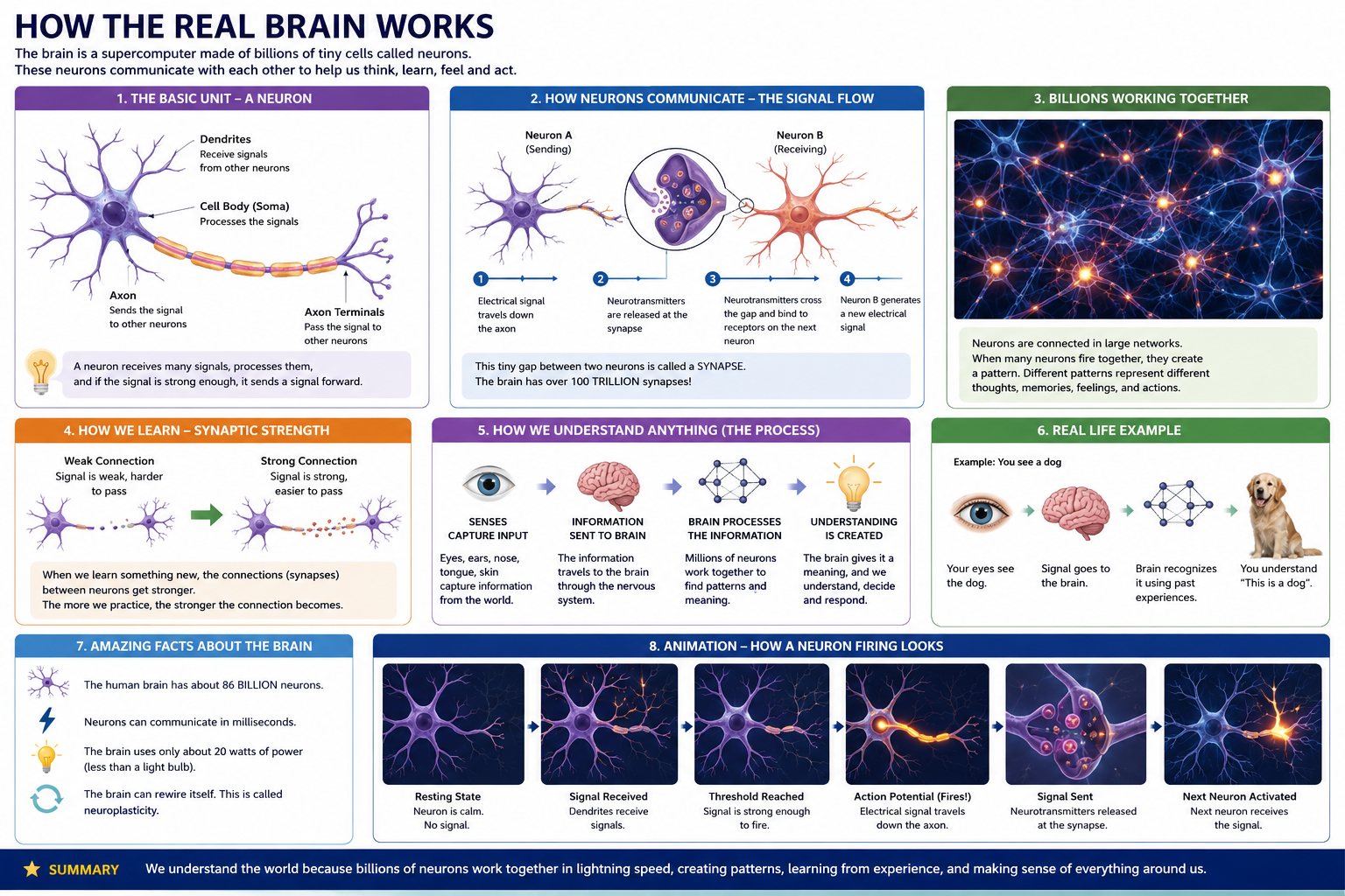
Look at panels 1, 4 and 8 of the infographic in particular. They contain the three ideas that artificial neural networks copy:
Many inputs, one decision
A neuron collects signals from many dendrites and fires only if the total is strong enough (panel 1 and 8, “threshold reached”).
Connection strength
Some connections are strong, some weak (panel 4). In a network these strengths are called weights.
Learning = changing strengths
Practice makes useful connections stronger. Training a network does exactly this: it adjusts the weights.
The artificial neuron
An artificial neuron is a tiny piece of maths that mimics a brain cell. It does exactly two things, in order:
- Linear step:
z = w·x + b, a weighted sum of the inputs plus a bias. - Non-linear step:
a = activation(z), which decides how strongly the neuron “fires”.
| Real brain | Artificial neural network |
|---|---|
| Dendrites receive signals | Inputs x₁, x₂, x₃ … |
| Synapse strength | Weights w₁, w₂, w₃ … |
| Cell body combines signals | Weighted sum z = w·x + b |
| Fires only above a threshold | Activation function |
| Axon passes the signal on | Output a, which becomes input to the next layer |
| Learning strengthens synapses | Training adjusts the weights |
Inputs x = [2, 3], weights w = [0.5, −1], bias b = 1. What is z? What does ReLU output?
Show the working
z = (2 × 0.5) + (3 × −1) + 1 = 1 − 3 + 1 = −1. ReLU(−1) = max(0, −1) = 0, so this neuron stays silent. A sigmoid would output about 0.27 instead.
Stack many neurons side by side and you get a layer. Stack layers and you get a network. “Deep” simply means many layers.
Without step 2, no matter how many layers you stack, the whole network collapses mathematically into one big linear function: a straight line. Non-linearity is what lets a network bend its decision boundary into curves and learn complex shapes.
Why deep learning exists at all
Classical ML needs a human to hand-craft the features, such as “edge detector” or “word frequency”. Deep learning's big idea is representation learning: stack enough layers and the network discovers its own features, layer by layer.
In vision
In text
The only maths you need to start
Three ideas, used over and over at huge scale:
- Linear algebra. A vector is one row of features, a matrix is a set of weights, and the dot product is a weighted sum: the core operation in every layer.
- Calculus. A derivative answers “if I nudge this weight a little, how much does the error change?” That question is the entire engine of training.
- Probability. A model's output is usually a probability distribution. A loss function measures how far that predicted distribution is from the true one.
Classical ML in one table
| Concept | What it means |
|---|---|
| Supervised learning | Learn f(x) → y from labelled examples. Regression: y is a number. Classification: y is a category. |
| Unsupervised learning | Find structure with no labels: clustering, dimensionality reduction. |
| Bias–variance trade-off | Underfitting (too simple, high bias) vs overfitting (memorises noise, high variance). The central tension in all of ML. |
| Core algorithms | Linear/logistic regression → decision trees → random forest and gradient boosting → SVM, KNN. |
| Evaluation | Classification: accuracy, precision, recall, F1, ROC-AUC. Regression: RMSE, MAE, R². Always check on data the model hasn't seen (train/validation/test split or k-fold cross-validation). |
Activation functions, and why ReLU won
- Sigmoid and tanh squash values into a fixed range, but their slope is almost zero at the extremes. In deep stacks, the learning signal shrinks to nothing as it travels backward. This vanishing gradient problem nearly stalled deep learning in the 1990s and 2000s.
- ReLU,
max(0, z), has a slope of either 0 or 1, so the signal doesn't shrink. This simple fix is a big reason deep learning became practical after 2012. - GELU and SiLU are smoother versions of ReLU used in modern Transformers like GPT and BERT, because they perform slightly better at scale.
Loss functions: measuring the mistake
MSE (mean squared error)
For regression. Squares each error, so big mistakes are punished much more than small ones.
Cross-entropy
For classification. Measures how wrong a predicted probability distribution is compared with the true answer. Pairs with sigmoid (two classes) or softmax (many classes).
How a network learns: gradient descent and backpropagation
Imagine the loss as a hilly landscape. Each weight is one direction you can walk in, and the height is the error. Training is a ball rolling downhill. The gradient tells you which way is downhill from where you stand: take a step, recompute the slope, step again.
Backpropagation is how the network finds the slope for every single weight. It is just the chain rule from calculus, applied layer by layer:
- Compute the loss at the output.
- Ask: how much did each weight in the last layer contribute to that loss? (A direct derivative.)
- Ask the same for the layer before, using how much the last layer's inputs mattered (chain rule again).
- Continue backward to the first layer. Then update every weight a little, downhill.
There is no magic. It is careful bookkeeping, and frameworks like PyTorch do it for you automatically.
Optimisers: choosing the step intelligently
| Optimiser | Idea |
|---|---|
| SGD | Plain gradient descent. Simple, but can be slow and zig-zag in narrow valleys. |
| SGD + momentum | Keeps a “velocity” so it doesn't zig-zag: a heavy ball instead of a light pebble. |
| Adam | The modern default. Adapts the learning rate for each weight using running averages of past gradients. |
| Learning-rate schedules | Start higher and decay over time (warm-up, cosine, step decay). This often matters more for final accuracy than people expect. |
Regularisation: fighting overfitting
| Technique | What it does |
|---|---|
| Dropout | Randomly switches off neurons during training, forcing the network not to rely on any single path. |
| Batch normalisation | Normalises activations layer by layer, which stabilises and speeds up training. |
| Weight decay (L2) | Penalises large weights, giving simpler, smoother functions. |
| Early stopping | Stop when validation loss stops improving, even if training loss keeps falling. |
| Data augmentation | Create extra training data with crops, flips and noise. The cheapest regulariser there is. |
Architectures: same building blocks, different wiring
MLP
Fully connected layers. Good for tabular data and the foundation everything else builds on.
CNN
Slides small filters across an image to detect local patterns. A cat's ear looks like a cat's ear wherever it is in the picture. More in Computer Vision.
RNN, LSTM, GRU
Process sequences step by step, carrying a memory forward. Largely replaced by Transformers for language.
Transformer
Every token looks at every other token at once through self-attention, so it trains in parallel on GPUs. The backbone of every modern LLM. More in Transformers.
Autoencoders, GANs, diffusion
Generative architectures that compress-and-rebuild or create realistic new samples. GANs and VAEs have their own lessons.
What it looks like in real code
Professionals don't write backpropagation by hand. They use a framework such as PyTorch, which computes every gradient automatically (autograd). Here is a small network that learns to separate two interleaving “moon” shapes. Read the four numbered comments: they are the whole training loop.
# pip install torch scikit-learn
import torch
from torch import nn
from sklearn.datasets import make_moons
from sklearn.model_selection import train_test_split

X, y = make_moons(n_samples=2000, noise=0.2, random_state=42)
X_tr, X_val, y_tr, y_val = train_test_split(X, y, test_size=0.2, random_state=42)
X_tr, X_val = torch.tensor(X_tr, dtype=torch.float32), torch.tensor(X_val, dtype=torch.float32)
y_tr = torch.tensor(y_tr, dtype=torch.float32).unsqueeze(1)
y_val = torch.tensor(y_val, dtype=torch.float32).unsqueeze(1)

model = nn.Sequential(          # 2 inputs → two hidden layers → 1 output
    nn.Linear(2, 32), nn.ReLU(),
    nn.Linear(32, 32), nn.ReLU(),
    nn.Linear(32, 1),
)
loss_fn = nn.BCEWithLogitsLoss()                      # cross-entropy for 2 classes
optimizer = torch.optim.Adam(model.parameters(), lr=0.01)

for epoch in range(200):
    model.train()
    optimizer.zero_grad()
    loss = loss_fn(model(X_tr), y_tr)   # 1. forward pass  2. measure the loss
    loss.backward()                     # 3. backpropagation (autograd)
    optimizer.step()                    # 4. update the weights

    if epoch % 20 == 0:
        model.eval()
        with torch.no_grad():           # inference: no gradients needed
            acc = ((model(X_val) > 0).float() == y_val).float().mean().item()
        print(f"epoch {epoch:3d}  loss {loss.item():.3f}  val accuracy {acc:.1%}")
Compare this with the steps above: forward pass, loss, backward pass, weight update. Notice the torch.no_grad() block: that is inference, running the model without learning.
Thinking like a professional
Building a model that learns is the start. These habits separate a model you can trust from one that only looks good in a notebook:
- Diagnose with learning curves. Plot training vs validation loss. Both high → underfitting (use a bigger model). Training low but validation high → overfitting (more regularisation or data). Both low and close → good.
- Search hyperparameters systematically. Grid search for small spaces, random search for bigger ones, Bayesian tools like Optuna when each run is expensive.
- Batch size and learning rate are linked. Bigger batches usually want bigger learning rates.
- Use mixed precision (fp16/bf16). Roughly twice as fast on modern GPUs with negligible accuracy loss.
- Data is usually the bottleneck, not architecture. Cleaning labels, fixing class imbalance and adding better examples beats architecture tweaks most of the time.
- Plan for production. Export (ONNX, TorchScript), shrink with quantisation (fp32 → int8), version both models and data, and monitor for drift: real-world data slowly changing away from what the model was trained on.
Key takeaways
- An artificial neuron = weighted sum + activation, inspired by how brain cells fire.
- Networks learn by gradient descent: measure the loss, find the slope with backpropagation, step downhill.
- ReLU, Adam and regularisation are what made deep networks practical to train.
- Different architectures (CNN, RNN, Transformer) are the same building blocks wired for different data.
Check your understanding
1. In an artificial neuron, what plays the role of synapse strength?
Weights scale each input, just as stronger synapses pass stronger signals. Training adjusts them.
2. What happens if you remove all activation functions from a deep network?
Stacked linear steps are still linear. Non-linearity is what gives depth its power.
3. Training loss keeps falling but validation loss starts rising. What is happening?
The model is memorising the training data. Try early stopping, dropout, weight decay or more data.
4. Why did ReLU help deep learning take off?
Sigmoid and tanh have near-zero slopes at the extremes; ReLU's slope is 0 or 1, so the learning signal survives many layers.